Variance — the statistical name for "divisive"
Every argument about a "polarizing winner" is an argument about spread, and spread has a name and a formula. This page gives it both, runs the smallest election where spread is the only thing separating two candidates, and then points at the trap that makes raw variance a worse divisiveness score than it looks: on a bounded 0–5 ballot, how much variance a candidate can even have depends on their average. Expanded from the statistics you actually need, which introduces the idea in a paragraph.
Level: 201 → 301 · deep dive Companions: distribution shape · the majority criterion — where this argument is actually fought · does a better ballot end polarization? — the reform claim built on top of it.
The definition, and why a rated ballot is what makes it available
Variance is the average squared distance from the mean; standard deviation is its square root, back in the units of the ballot. Low variance means the scores bunch; high variance means they fly apart. That is the entire idea.
What matters for voting is not the formula but the input. Variance needs numbers on a shared scale, so it exists for a score ballot and does not exist for a ranked one. A ranking records that voters disagreed about the order; it cannot record how far apart they were, because "1st > 2nd" is the same mark whether the gap was a hair or a chasm (scores vs. ranks). So "this candidate is divisive" is a claim a rated ballot can make arithmetically and a ranked ballot can only make by inference.
One election where spread is the only difference
Two candidates, five voters. Alice is a flat 3 on every ballot. Blake takes three 5s and two 0s. Both total 15; both average 3.0. The score distribution is the whole story:
The ballots as marked — the filled bubble is the score given, and the score is the number in its column:
| # | Ballot as marked | Alice | Blake |
|---|---|---|---|
| 1 | 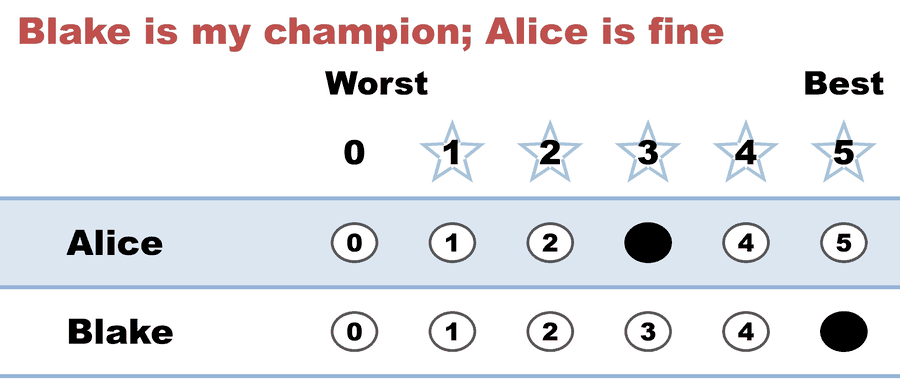 |
3 | 5 |
| 2 | 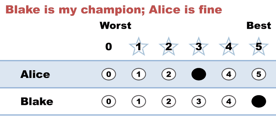 |
3 | 5 |
| 3 | 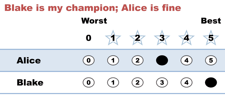 |
3 | 5 |
| 4 | 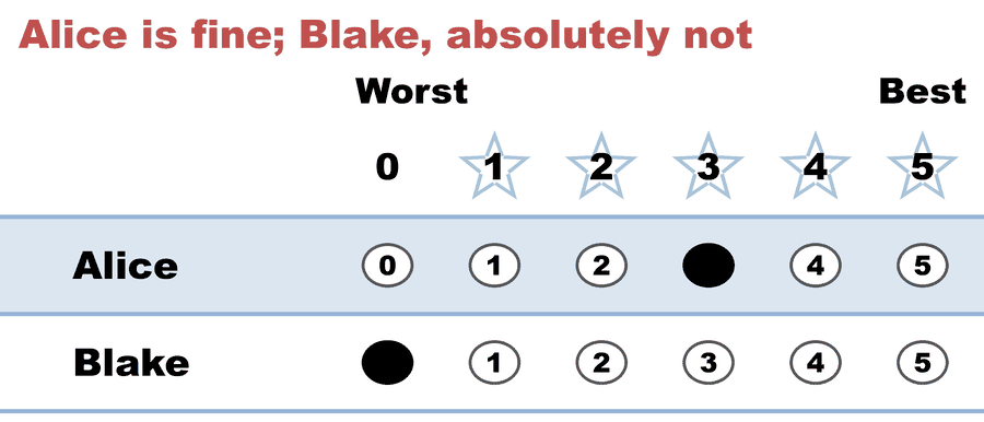 |
3 | 0 |
| 5 | 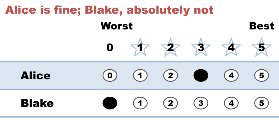 |
3 | 0 |
[Divergence from STAR]
  STAR     = Blake
  Approval = Alice   (differs from STAR)

--- STAR Voting Method (single winner) ---

[STAR Voting]
 Tabulating 5 ballots.
Count × Alice,Blake
    3 ×     3,    5
    2 ×     3,    0

[STAR Voting: Scoring Round]
 The two highest-scoring candidates advance to the next round.
   Alice         -- 15 -- First place
   Blake         -- 15 -- Second place
 Alice and Blake advance.

[STAR Voting: Automatic Runoff Round]
 The candidate preferred in the most head-to-head matchups wins.
   Blake         -- 3 -- First place
   Alice         -- 2
   Equal Support -- 0
 Blake wins.
   Runoff math:
     5  ballots cast
   − 0  Equal Support (no preference between the two finalists)
     ─
     5  voters with a preference  (majority = 3)
           Blake 3 (60%)  ·  Alice 2 (40%)

[STAR Voting: Winner — STAR Voting Method (single winner)]
 Blake
Same mean, variance 0.0 vs 6.0 (standard deviation 0.00 vs 2.45). And the methods do not agree about what to do with that:
| Method | Winner | Why |
|---|---|---|
| Score / Range | tie, 15–15 | the total is all it reads, and the totals are identical — the seat falls to a tie-break, which is not the same thing as choosing |
| Approval (approve = 3+ stars, the reading the engine's divergence block uses) | Alice 5–3 | a flat 3 clears the bar on every ballot; Blake's 0s clear nothing |
| STAR | Blake 3–2 | the automatic runoff reads the order inside the scores, and 3 of 5 rank Blake above Alice |
| RCV-IRV · Ranked Robin · Choose-One | Blake | Blake holds 3 of 5 first choices — an outright majority in round one |
Full count, matrix and audit: the generated case page. Every method side by side: its entry in the divergence ledger, which reports the Score row as Alice because it settles the 15–15 tie by ballot-column order — worth knowing before the two pages look like they disagree.
Two honest notes on that table before it gets quoted. The engine flags Alice as the Condorcet loser — true, and much less dramatic than it sounds: with only two candidates there is exactly one head-to-head, so whoever loses it is simultaneously the Condorcet loser and the runner-up. And STAR "passing" here proves nothing general, because with two candidates STAR is majority rule; STAR genuinely does fail the majority criterion, and it takes a third candidate to show it.
The arithmetic trap: you cannot tie a flat 3 with a half-and-half split
The stock illustration of this idea — "one got 3s from everybody, the other got 5s from half the electorate and 0s from the other half, same mean" — does not tie. Half 5s and half 0s averages 2.5, not 3.0, and no flat integer score on a 0–5 ballot averages 2.5. The comparison only works if you move one side:
| Consensus candidate | Polarizing candidate | Mean | Ties? |
|---|---|---|---|
| flat 3 | 5s from half, 0s from half | 3.0 vs 2.5 | ✗ |
| flat 3 | 5s from three voters in five, 0s from the other two | 3.0 vs 3.0 | ✓ (the case above) |
| flat 3 | 5s from half, 1s from half | 3.0 vs 3.0 | ✓ (less vivid — nobody is at rock bottom) |
| half 2s / half 3s | 5s from half, 0s from half | 2.5 vs 2.5 | ✓ (no flat score, but it ties) |
Widening the scale is not the escape hatch it looks like: pairing a flat 3 with "6s from half" ties the mean only on a ballot that has a 6, and a STAR ballot does not. Changing the scale is never free either — it can move the winner, not just the arithmetic (scale granularity can flip the winner). Fix the split, not the scale.
The trap that matters more: on a bounded ballot, variance depends on the mean
This is the part that is genuinely under-appreciated, and it undercuts the casual use of variance as a divisiveness score.
Scores live in [0, 5]. A bounded variable cannot have arbitrary spread — and the ceiling moves with the average. For a distribution on [0, M] with mean m, the Bhatia–Davis inequality caps the variance at m(M − m), reached only by putting every voter at one of the two ends. On a 0–5 ballot:
| Average score | Max possible variance | Max possible SD |
|---|---|---|
| 0.5 | 2.25 | 1.50 |
| 1.0 | 4.00 | 2.00 |
| 2.0 | 6.00 | 2.45 |
| 2.5 | 6.25 | 2.50 |
| 3.0 | 6.00 | 2.45 |
| 4.0 | 4.00 | 2.00 |
| 4.5 | 2.25 | 1.50 |
Three consequences, and each one bites a real argument:
- Blake, above, is maxed out. At a mean of 3.0 the ceiling is exactly 6.0, and Blake sits on it — he is precisely as divisive as a 0–5 ballot permits at that average. That is a sharper statement than "high variance," and it is checkable.
- A well-liked candidate cannot look divisive, however split the electorate is. A candidate averaging 4.5 caps at variance 2.25, less than half Blake's — even if every single voter is at an extreme (here, 90% giving 5 and 10% giving 0). Rank candidates by raw variance and you have partly ranked them by how mediocre their average is.
- Peak measurable divisiveness sits at the middle of the scale, mean 2.5. So the statistic is not neutral about where on the ballot the fight happens.
If you want a number that isn't confounded, divide by the ceiling — variance / (m(5 − m)), a 0-to-1 share of the maximum spread available at that average. Blake scores 1.00; Alice 0.00. (That ratio is this page's shorthand for a fix, not a term of art in the literature — say what you computed when you quote it.) The lower-tech option is usually better anyway: report the distribution instead of a summary of it. The engine's Score Distribution block — always in the _tabulated mirror and the generated case page, or on screen with --full — prints the whole shape, and "3 fives, 2 zeros, nothing in between" argues better than any single statistic.
What variance does not do
No method in this library counts it. Variance is a lens on the ballots, not a step in any tabulation here — STAR, Score, Approval and Majority Judgment all respond to spread, but none of them computes it. What they differ on is which part of the distribution their rule happens to be sensitive to: a sum is dragged by the extremes, a median ignores how extreme they are, an approval threshold sees only which side of one line each score falls on. Sensitivity to spread is a consequence of the counting rule, never an input to it. Any claim that a method "penalizes divisive candidates" has to name the mechanism that does it.
And high variance is not a defect. A reformer with a real mandate and real opponents is high-variance; so is an incumbent in a genuinely split electorate. Variance measures how concentrated opinion is, not whether electing that person is a good idea — that judgment belongs to the values question, not to the statistic. "Divisive" is what the number is; whether divisive should lose is what the argument is about.
Where the argument actually lives
Strip the statistics away and the disagreement is one question: should a majority's intensity outrank a minority's rejection? Every camp answers by pointing at a distribution.
- The consensus case — a candidate 40% of voters score at rock bottom represents fewer people than one nobody objects to. Worked in full at the majority criterion (STAR electing broadly-liked Bruno over majority-favorite Ada) and in the Black Curtain set, whose Election 3 is this page's election with the means untied: the "landslide" winner is zeroed by 40% of voters while a rival is liked by all five.
- The majority case — a group that is more than half of the electorate and prefers a candidate should get that candidate, and calling their winner "divisive" is a way of not counting them. This is the objection FairVote presses hardest, and it is the reason STAR has a second round at all.
- The measurement case — that neither side should be arguing from a mean in the first place, because the mean threw the shape away before the argument started. That one is this page.
Which candidate wins under a given method is then a question about that method's rule, not about the variance: see majority & minority candidates for the five different things "majority candidate" can mean, and STAR's honest limits for where STAR pays for its answer.
Related
- The statistics you actually need — this idea in one paragraph, alongside mean-vs-median, sum-vs-mean, and correlation
- Preference vs. support — the ballot-level distinction that makes spread recordable at all
- Cardinal utility — what the number in the bubble is reaching for, and why summing it needs more than "it's a number"
- Center squeeze — the low-variance candidate's characteristic way of losing under IRV
- The spatial voting model · election simulation models — where these distributions come from in simulation
- Range voting · Approval — the two methods this election separates most sharply